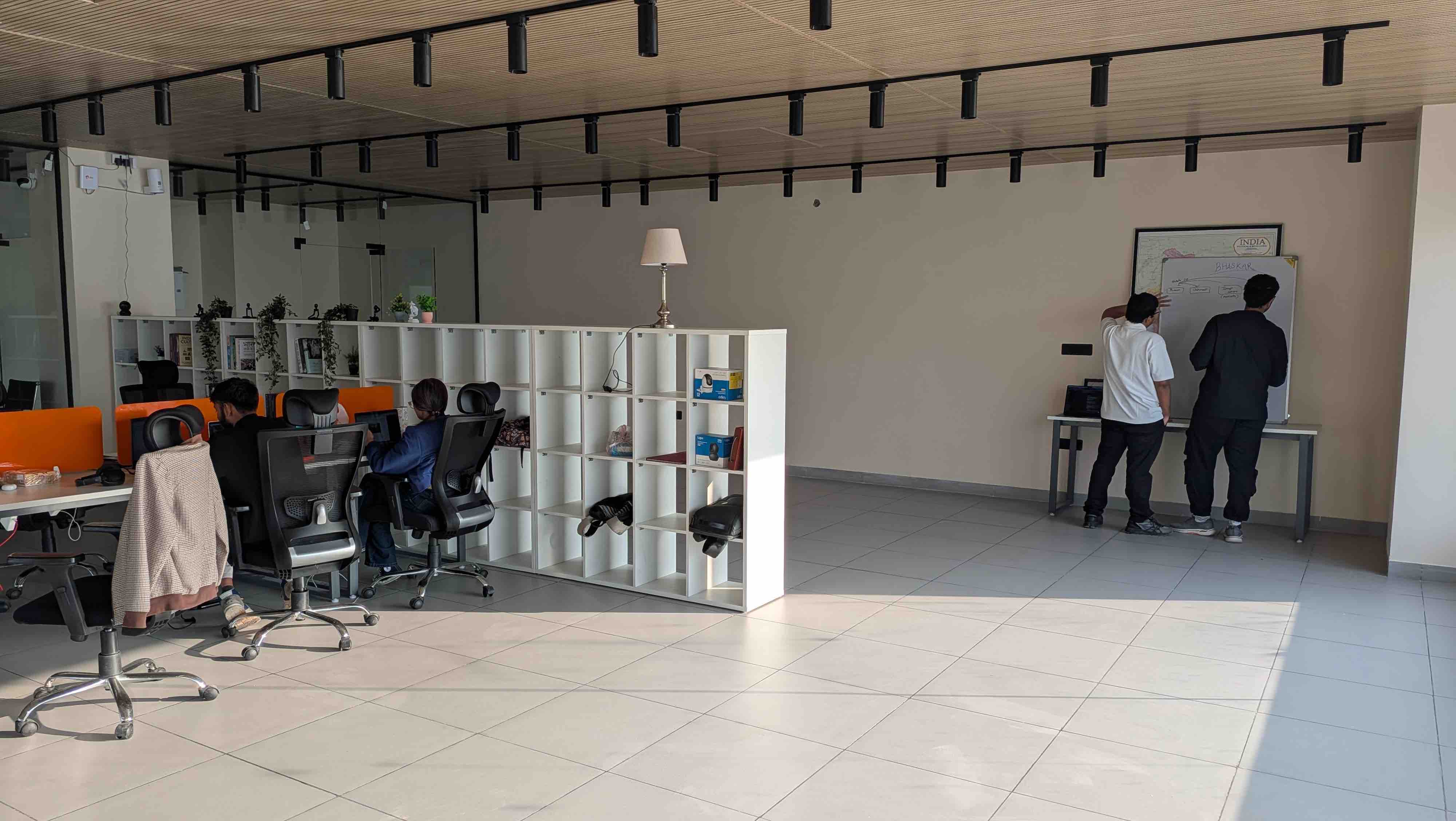
Case Study: How Chhaon Was Built to Turn Shade Into Infrastructure You Can Measure

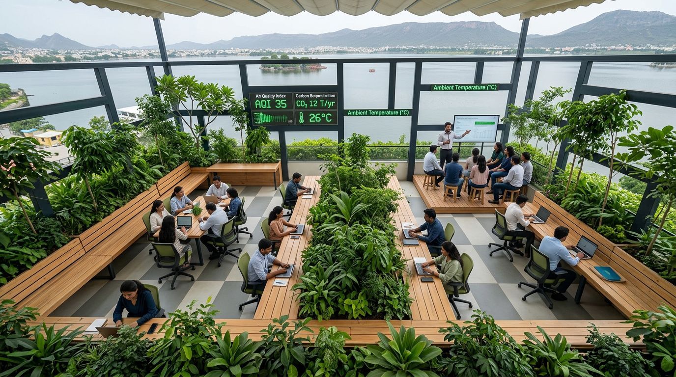
Executive Summary

Ajmer's streets hit 46 to 50 degrees Celsius every summer. Everyone in the city knows a tree gives you relief. Almost nobody can tell you how much. That gap between what people feel and what anyone can prove is the reason Chhaon exists

Chhaon is a climate tech project by Project Bhaskar, built at Ana Sagar in Ajmer, Rajasthan. It's three things under one roof: a forest grown using the Miyawaki method, a co-working space built as climate tech infrastructure with no air conditioning, and a library. A quiet sensor network runs underneath all three, tracking temperature, humidity, carbon dioxide, air quality, and soil moisture around the clock. It's a forest you can sit inside, and it's also a working scientific instrument.

This case study covers how that instrument got built — a plant list, a prototype building, a storm that ruined a sensor, and a lot of small decisions that added up to something real. The hardware and the software described here are built and running today. The public dashboard, the wider multi-city vision, and any real carbon credit submissions are next steps, not finished results, and this piece says so plainly wherever that distinction matters.

The Challenge

Ajmer's peak summer temperature isn't a freak reading. Streets touch 46 to 50 degrees Celsius, and there's nowhere in the city to check whether any specific patch of shade is actually helping.

Part of the reason cities like Ajmer run this hot has a name: the urban heat island effect. Concrete and asphalt soak up heat all day, then release it slowly, well after the sun goes down. Trees don't work that way. They cool as they breathe. Tier-2 Indian cities, Ajmer included, run 4 to 6 degrees hotter than the open country just outside their limits, because they have lost close to 30 percent of their tree cover since 2001. That number matters because one mature tree can cool the air around it by 2 to 8 degrees, just through evapotranspiration, which is the process of a tree pulling water up through its roots and releasing it as vapor through its leaves. A tree also gives rain somewhere to land and soak into the ground, instead of running straight off hot pavement into a drain.

Ana Sagar Lake, adjacent to the Chhaon site, illustrates a related environmental challenge: urban heat and water systems are closely interconnected. The lake has faced long-standing pressures from water quality degradation, catchment modification, and encroachment, making it a useful indicator of the broader ecological stresses affecting Ajmer.

These systems reinforce one another. Higher ambient temperatures increase evapotranspiration, accelerating moisture loss from soils and vegetation. Reduced soil moisture, in turn, weakens the natural cooling provided by evapotranspiration, creating a feedback loop that intensifies local heat exposure.

The impacts are not distributed evenly. Outdoor workers, street vendors, informal-sector labourers, schoolchildren, and others who spend prolonged periods in public spaces experience the greatest exposure to elevated temperatures while often having the fewest options for thermal refuge.

This exposes a broader evidence gap. Although the cooling benefits of urban vegetation are well established in scientific literature, Ajmer currently lacks publicly available, site-specific data that quantifies the cooling performance of urban green infrastructure under local conditions. Chhaon's primary objective is therefore not only to create a cooler public space, but also to generate continuous, verifiable environmental measurements that demonstrate and quantify those benefits in a real urban setting.

Why Chhaon Was Needed

Rajasthan's ecological history influenced several of Chhaon's core design decisions. One of the most significant lessons comes from the introduction of Prosopis juliflora, a non-native shrub that was widely planted across the state during the twentieth century to combat desertification. Although intended to stabilise degraded land, the species spread aggressively, displaced native vegetation, altered soil conditions, and reduced local biodiversity. In many areas, landscapes appeared greener from above while becoming ecologically less diverse on the ground.

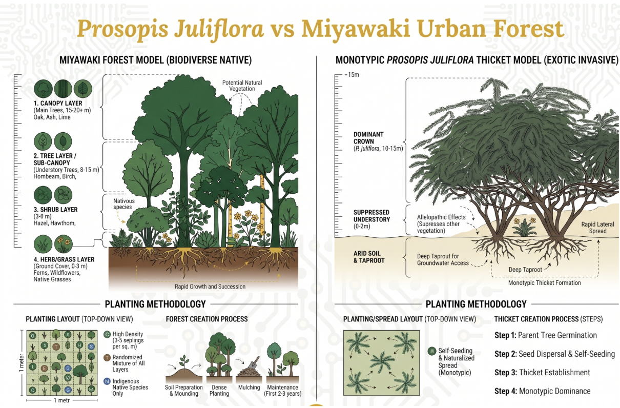
Figure 1 — Comparison of Prosopis juliflora and Miyawaki style forest plantation.

That's the cautionary tale behind Chhaon's rule that every plant has to be native (as far as possible) - nothing imported, nothing that looks good from a drone shot and does nothing for the ground underneath it.

Existing environmental monitoring systems also presented a different limitation. Most commercially available sensor platforms are designed to measure ambient environmental conditions at a single location. They are not intended to continuously compare paired microclimates — for example, conditions inside a forest canopy against those on an adjacent paved street — using synchronised, publicly accessible measurements. This comparative capability became a core design requirement for Chhaon.

At the time Chhaon was conceived, Ajmer had no publicly accessible, continuously measured demonstration of the cooling performance of urban vegetation.

The Solution

Three physical parts share the same site: a forest grown using the Miyawaki method, a co-working space built as climate tech infrastructure with no air conditioning, and a library next to both. Earlier project materials describe the second part as a café. Today the team runs it closer to a membership knowledge space, cooled by the forest instead of a compressor, and that framing is still settling as the project grows.

The project's own language puts it better than any summary could: this is not a café with some plants around it, it's a climate experiment you can sit inside of.

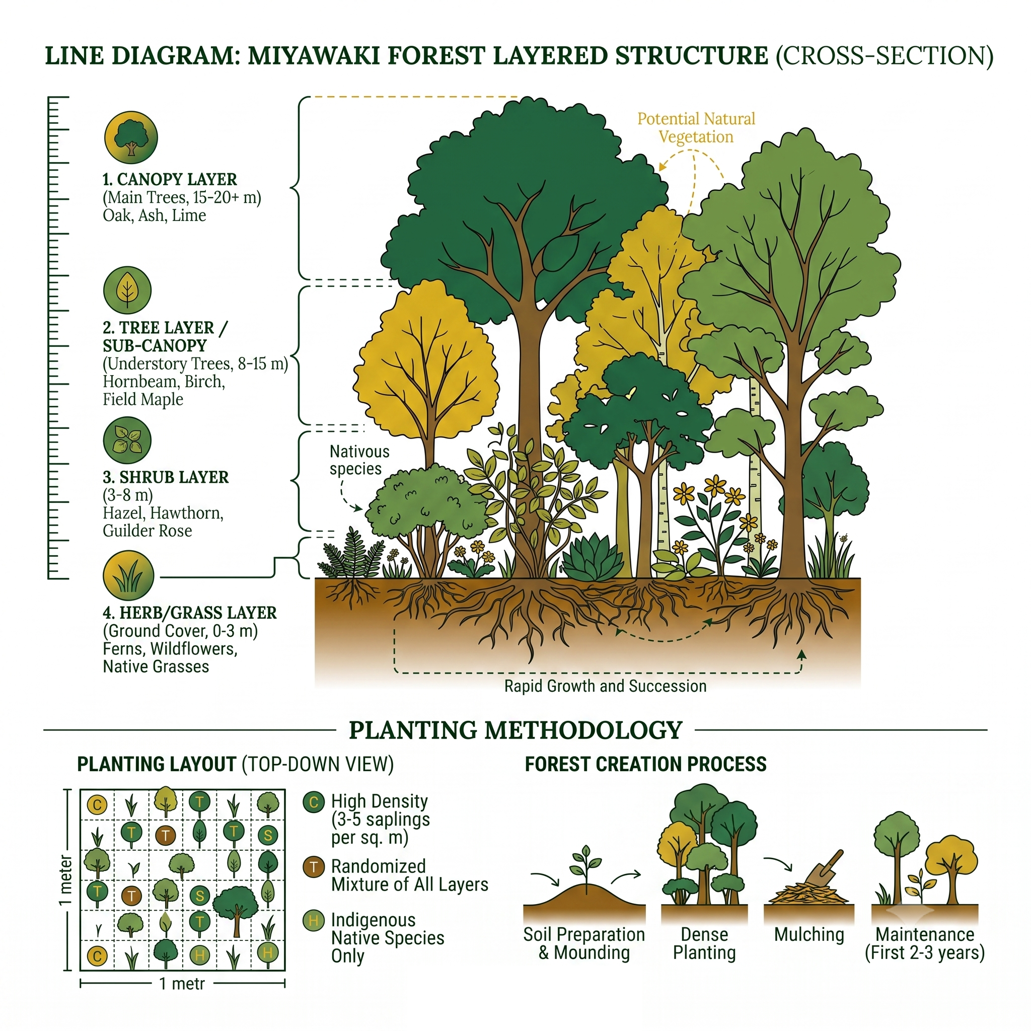
Figure 2 — Line diagram of Miyawaki Forest planting method and how it grows.

What ties the whole site together is the sensor layer running underneath it. Every part of the forest that gets planted is also being measured, so "shade is infrastructure" isn't just a line on a wall. It's something you can pull up on a screen.

Forest Plantation and Challenges

The Miyawaki method is a way of planting a forest so dense and so layered that it grows many times faster than a normal plantation. It works in three layers at once. The canopy layer is made of the tallest native trees, the ones that will eventually form the roof of the forest. Below that sits the shrub layer, smaller native bushes that fill the middle space. Below that is the grass layer, low ground cover that closes off the soil.

At Chhaon, all three layers go into the same container at the same time — packed close together, instead of one layer spread over years. The containers themselves sit on a cemented floor, not bare ground, because the site is built on a rooftop, five floors up. Planting all three layers together forces the young trees into fierce competition for light from day one. Instead of growing wide and slow the way a lone tree does in an open field, they grow tall and fast, racing each other toward the sun. That competition, strange as it sounds, is exactly what makes a Miyawaki forest mature in years instead of decades.

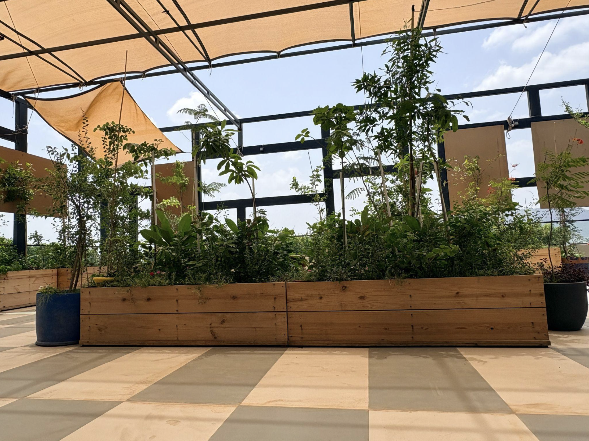
Figure 3 — All the containers placed at Chhaon.

Innovation and Challenges

Before any of this was built at scale, the team built one sample node first. It was a small drum, planted using the same three-layer Miyawaki technique, just to see what the method actually looked like in practice. That one drum turned out to be more convincing than expected. A friend who saw it got curious enough that the team sent it to him. So they built a second one, kept it on a terrace, and used it as their working reference for how the layers were supposed to look and behave before scaling up to the full site.

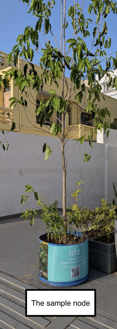
Figure 4 — The sample node that was first set-up and later sent to a friend.

Once the team understood the method well enough to build for real, they brought in a local carpenter to build roughly 12 to 13 containers over several days. After the containers were ready, a local mali (a gardener) came in to plant the trees, shrubs, and grass layers into each one.

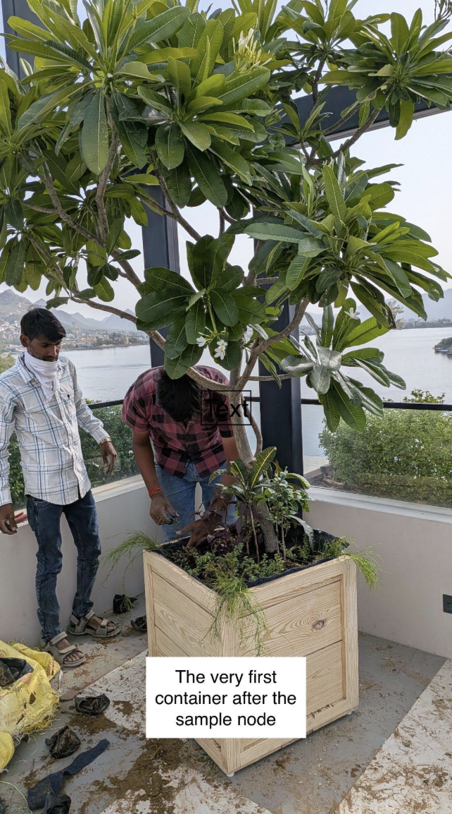
Figure 5 — The first container built; and the plantation starts.

Sourcing the plants themselves was its own fight. Picking the right main canopy trees, and then finding companion shrub and grass species that would actually thrive next to them, took real research. Ajmer's own nurseries didn't carry enough stock of the right native species, so the team ended up sourcing plants from nurseries in Pushkar instead, a short drive away.

Ajmer's heat brought its own problem. The containers needed shade above them just to keep the young plants alive through the peak months. The first attempt used a green shade net tied down with metal wire, and it didn't survive contact with Ajmer's windstorms and dust storms. The wire gave way and the shade came loose. The fix was to build a proper metal frame first, and only then stretch the green shade over it, instead of relying on wire alone.

Wind caused a second problem entirely. Because Chhaon sits on a fifth floor, open on both sides, wind pressure up there is nothing like wind at street level. Trees in the containers kept tipping and falling under that pressure. The team fixed it with rectangular wooden boards positioned to break the wind, plus bamboo stick supports staked next to each tree to hold it steady while its roots were still establishing.

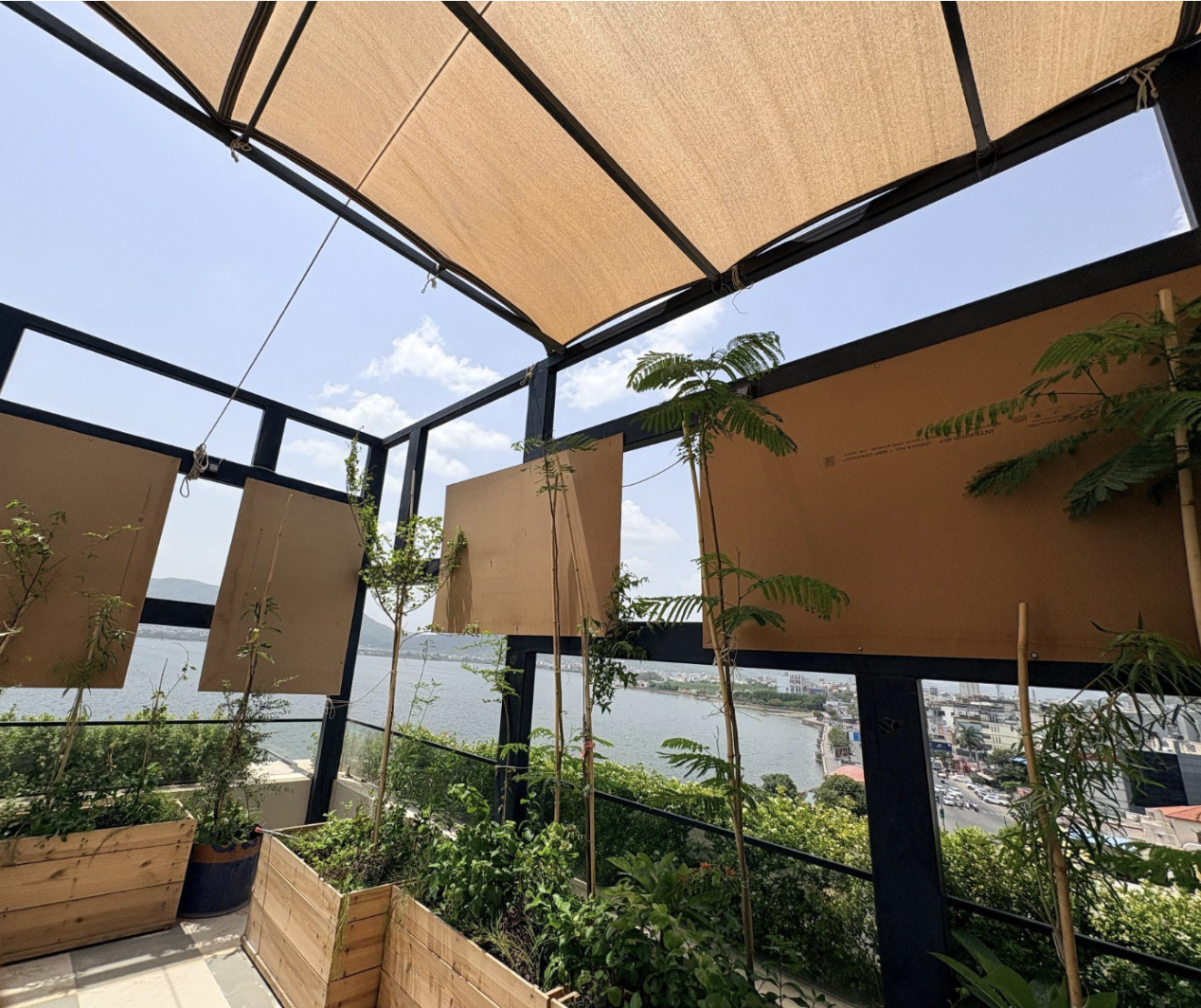
Figure 6 — The wooden boards hung to lower the impact of the strong winds during monsoon

Even the soil had a hidden problem. The containers were filled with a mix of soil, cocopeat, and fertiliser sourced locally, and that mix leaked water straight through hairline cracks in the container walls. The fix was almost embarrassingly simple: line every container with a rug before adding soil, cocopeat, and manure, so the water had nowhere to escape.

Concept Experience

This section describes how we currently imagine the Chhaon experience. It is an evolving concept rather than a final product, and many of the interactions described below are still being designed.

Imagine walking in from the Ana Sagar lakefront. You pass planting containers, each marked with a small QR code, into a shaded space where the usual hum of air conditioners is replaced by the cooling effect of the forest itself.

Visitors would become members through the Chhaon platform, selecting a membership tier that unlocks different ways to engage. We're exploring a system where live environmental readings—temperature, humidity and CO₂—appear directly on members' phones. A shared display within the space could compare the forest's conditions with those of the street outside, making the environmental impact visible in real time.

Beyond visiting, we're also imagining several ways people could contribute. Individuals and organisations might sponsor planting nodes through CSR partnerships, introduce collaborators who can help the project grow, or simply spend time in the space. Ultimately, Chhaon is intended to demonstrate, through lived experience and measurable data, what urban nature can do.

Technology

One reading on its own can't tell you whether the forest is doing something or the weather is, and thus Chhaon never trusts a single sensor to prove anything. Every Chhaon location will run two nodes instead of one - a canopy node planted inside the forest, and a reference node placed out on the street or rooftop nearby - reading the same things, at the same moment, a few metres apart.

Think of it like a control and a test group in an experiment. A single thermometer inside the forest can tell you it's 28 degrees in there right now - but 28 degrees could just mean it's a mild day everywhere. It's only once you also know it's 34 degrees on the street, at that exact same moment, that "28 inside" turns into "6 degrees cooler than the street" - a claim about the forest, not the weather. That comparison is the reason for the second node.

The two nodes will run mostly the same hardware, but not exactly the same, because they're not doing exactly the same job. Both will carry the same three core sensors - temperature, CO2, and air quality - since both need to measure the same things for the comparison to mean anything. From there, they diverge: the canopy node will also carry an e-paper screen and a touch sensor, because it's the one a visitor actually stands in front of and wants to read. On the other hand, the reference node will only a light sensor that te canopy node doesn't need, because it's the one whose job is to tell the backend how sunny it currently is outside the forest. Neither node is the "upgraded" one - they're built for two different jobs that only add up to something when read together.

The Sensors

Every Chhaon node will run four sensors, and each one earns its place for a specific reason

The BME280 handles temperature, humidity, and air pressure. It's the boring, reliable workhorse of the set, the sensor that just works and rarely needs a second thought.

The MH-Z19C measures carbon dioxide. This is the sensor that makes the "a forest breathes" idea measurable instead of poetic. It helps the CO2 gap between the air inside the canopy and the air out on the street.

The MQ-135 reads general air quality. Worth being honest about this one: it reports a relative trend, good, fair, or poor, not a lab-grade absolute number. Chhaon doesn't oversell what this sensor can say, and that honesty is part of the point.

The fourth is a capacitive soil moisture sensor, version 1.2, added to track how much water the containers are actually holding onto between waterings.

That's the shared core every node carries. But the canopy node and the reference node aren't identical - each one carries one extra piece of hardware the other doesn't need, matched to the job it's actually doing.

The reference node adds a VEML7700 light sensor. It isn't measuring light for anyone's comfort - it's there so the backend knows how much usable sunlight was actually falling on the site at any given moment. The carbon-capture math later in this document depends on this reading entirely: a CO2 gap measured at midnight isn't proof of anything, because the forest can't be photosynthesizing in the dark. The light reading is what lets the system tell those two situations apart.

The canopy node adds something that isn't a sensor at all: a TTP223 touch sensor, wired to the on-node e-paper screen. A single tap cycles the display through its three views - this node's own readings, the reference node's readings, and the two side by side - so anyone standing at the node can see the comparison for themselves, no app or login required.

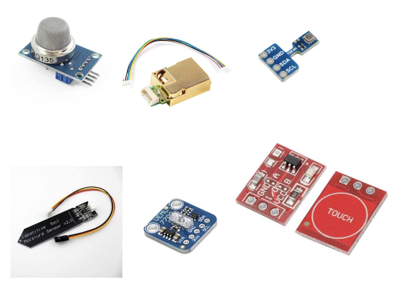
Figure 7 — MQ-135 (air quality)
Figure 8— MH-Z19C (CO2)
Figure 9 — BME280 (temperature, humidity, pressure)
Figure 10 — Capacitive soil moisture sensor v2.0
Figure 11 — VEML7700 (light / PAR — reference node only)
Figure 12 — TTP223 touch sensor (canopy node only — cycles the display)

From Wish List to Working Node

The original 2026 plan was ambitious. Three sensor nodes, each carrying eight or more sensor types: particulate matter, soil moisture at three separate depths, vibration detectors, motion sensors, even a camera. The budget for the plan ran ₹26,000 to ₹34,000.

A year later, one working node exists in the field — carrying the four sensors described above, powered over USB, sending a reading every 5 minutes. That's not a downgrade. It's what engineering maturity looks like: a team that chose to ship one honest, working instrument over a wish list that never left the page.

The brain of every node is an ESP32 DevKit v1, a small, inexpensive microcontroller with built-in WiFi and just enough processing power to run a field sensor without any fuss.

The Power Problem

The single biggest power draw inside a Chhaon node isn't the processor. It's the MQ-135 air quality sensor. Buried inside it is a small heating element that has to stay near 200 degrees Celsius, constantly, for the sensor's chemistry to work at all. That heater alone accounts for roughly half the node's entire power budget, running continuously rather than switching on and off.

The team's first instinct was solar power backed by a lithium battery — the setup you'd expect for an outdoor sensor. In practice, the two didn't pair well together for this build. The fix that actually shipped is simpler: a power bank connected to mains power, charging regularly, keeping the node running without the complexity a solar and battery pairing would have added.

From a Reading to a Number on a Screen

The path a single reading takes is short and deliberate: sensor, to ESP32, over WiFi, into InfluxDB, a time-series database built specifically for exactly this kind of stream of numbers, and from there onto a dashboard.

There's a decision worth calling out here. Most commercial IoT setups add a messaging layer in the middle, something like MQTT, to buffer and route data between devices and the cloud. Chhaon skipped that layer entirely and sent readings straight to the database. It's a scrappier choice, and a cheaper one. The whole pipeline runs on free-tier cloud tools instead of the thousands of rupees a month a commercial IoT platform would charge for the same job.

Turning Readings Into Meaning

This is the part of the system built to answer a harder question: not just "is it cooler in the forest," but "how much carbon is this forest actually pulling out of the air."

The math starts with the paired nodes. One sensor sits in the canopy, one sits out on the street as a reference point. Every reading, the system computes two gaps: the CO2 gap, reference reading minus forest reading, and the temperature gap, street minus canopy. A positive CO2 gap during the day means the forest air has less carbon in it than the street air, which is the forest doing its job.

Not every reading counts equally. Photosynthesis only happens with sunlight, so each reading gets weighted by how much usable light was available at that moment, capped at full weight once light crosses a known saturation point for most plants. A reading taken in full sun counts fully. A reading taken at dusk barely counts at all. A reading taken at night, when plants release CO2 instead of absorbing it, is expected to show a negative gap, and correctly counts for nothing rather than being treated as an error.

From there, the CO2 gap in parts per million gets converted into an actual weight, in kilograms, using the physical density of CO2 at that day's temperature and the measured volume of the canopy itself, area times height. As a worked example from the project's own engineering documents: an 85 square meter plot with a 2.1 meter canopy comes out to roughly 178.5 cubic meters of canopy volume. Feed a modest average gap through that formula across a full day of sunlight-weighted readings, and the math lands around 11 to 12 kilograms of captured CO2 a day, which would cross one full tonne in roughly three months. That's a demonstration of how the calculation works, not a confirmed measurement from the Ajmer site itself.

Weather is noisy, so the daily numbers get smoothed with a 7-day rolling average, and any single day that swings more than 15 percent past the trailing 30-day total gets capped, so one storm or one sensor hiccup can't distort the whole record. Before anything counts toward a credit, the system also checks that at least 85 percent of expected readings actually came in that period. A new site has to run for 60 days before any of its data is treated as credit-eligible at all, purely so the team can validate its own numbers before trusting them.

Where this actually stands today: this accounting system is real, working code, tested against real readings. Making any of it public, or submitting a real batch to a carbon registry, hasn't happened yet. That part is built, but it hasn't gone out the door.

Hardware Setup: Wiring the Node

Every Chhaon node is built around the same core: an ESP32 DevKit v1 wired to its sensors over I2C, UART, and a single analog pin, with the canopy node carrying an additional e-paper display and touch sensor that the reference node doesn't need. The table below is the actual pin-out from the node firmware.

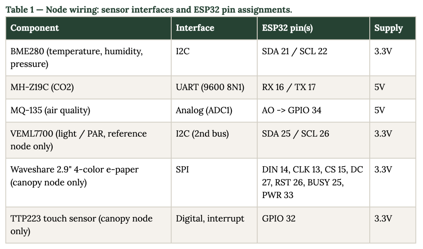
GPIO 34 is deliberately used for the MQ-135, not an arbitrary choice: it sits on the ESP32's ADC1 block, which is the only set of analog-capable pins that can still be read reliably while the WiFi radio is active. The ADC2 pins share hardware with the WiFi driver and give unreliable readings the moment the radio keys up - a detail that only shows up once you're debugging noisy sensor data in the field.

Each sensor also has its own personality that the firmware has to work around:

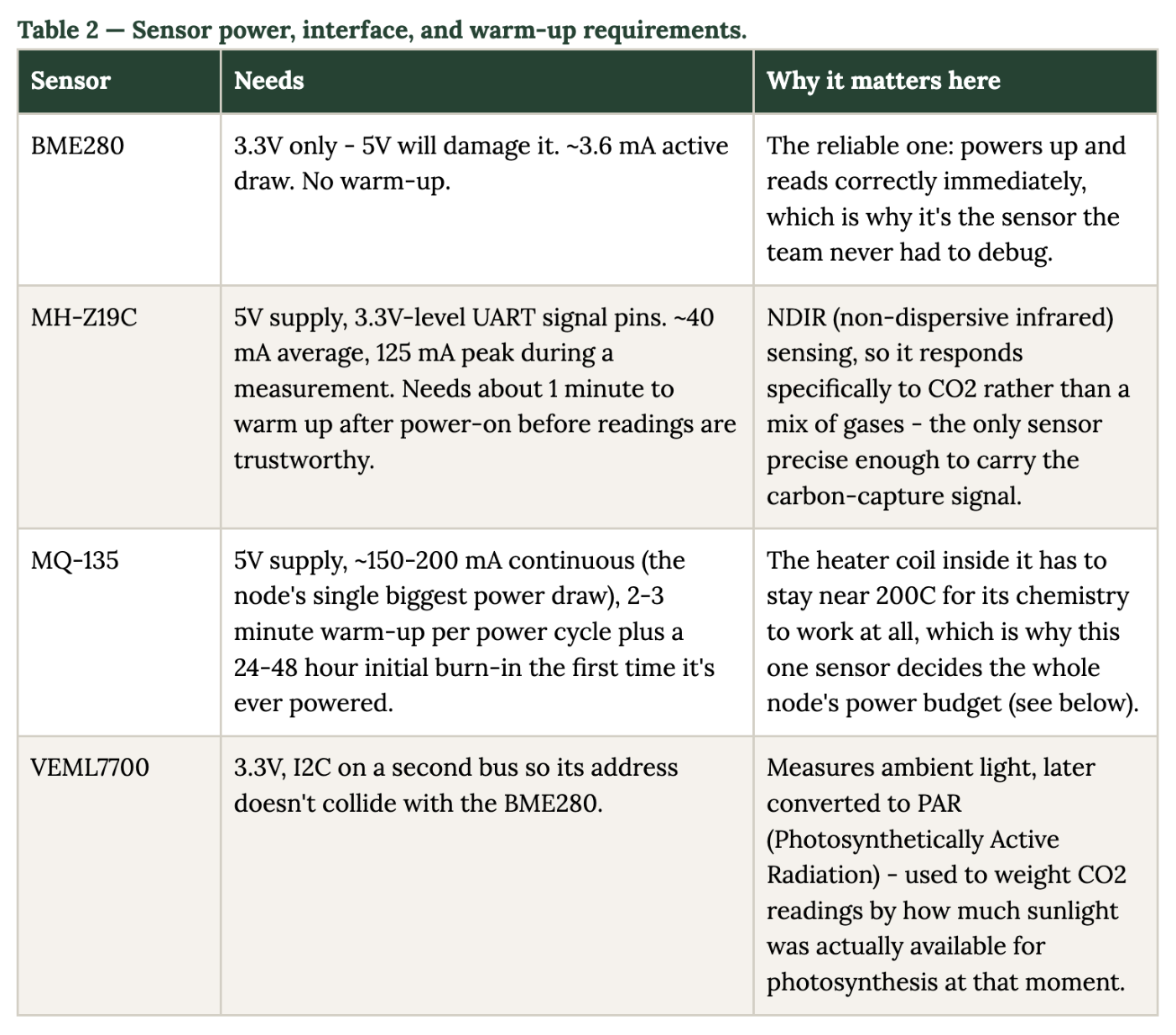
The MH-Z19C also carries a firmware-level detail worth calling out because it's the kind of thing that silently corrupts data if missed: the sensor's Automatic Baseline Correction (ABC) assumes the lowest reading it sees every 24 hours is clean outdoor air near 400 ppm, and quietly recalibrates itself against that assumption. Inside a dense canopy at midday, CO2 legitimately drops below 400 ppm because the forest is actively pulling it down - which would trick ABC into recalibrating against the wrong baseline. The canopy node's firmware explicitly disables ABC (mhz19.autoCalibration(false)) for exactly this reason, while the reference node - which always sits in open ambient air where the ABC assumption is actually true - leaves it enabled (mhz19.autoCalibration(true)). Getting this one flag backwards on either node would quietly poison every CO2 reading it ever produced.

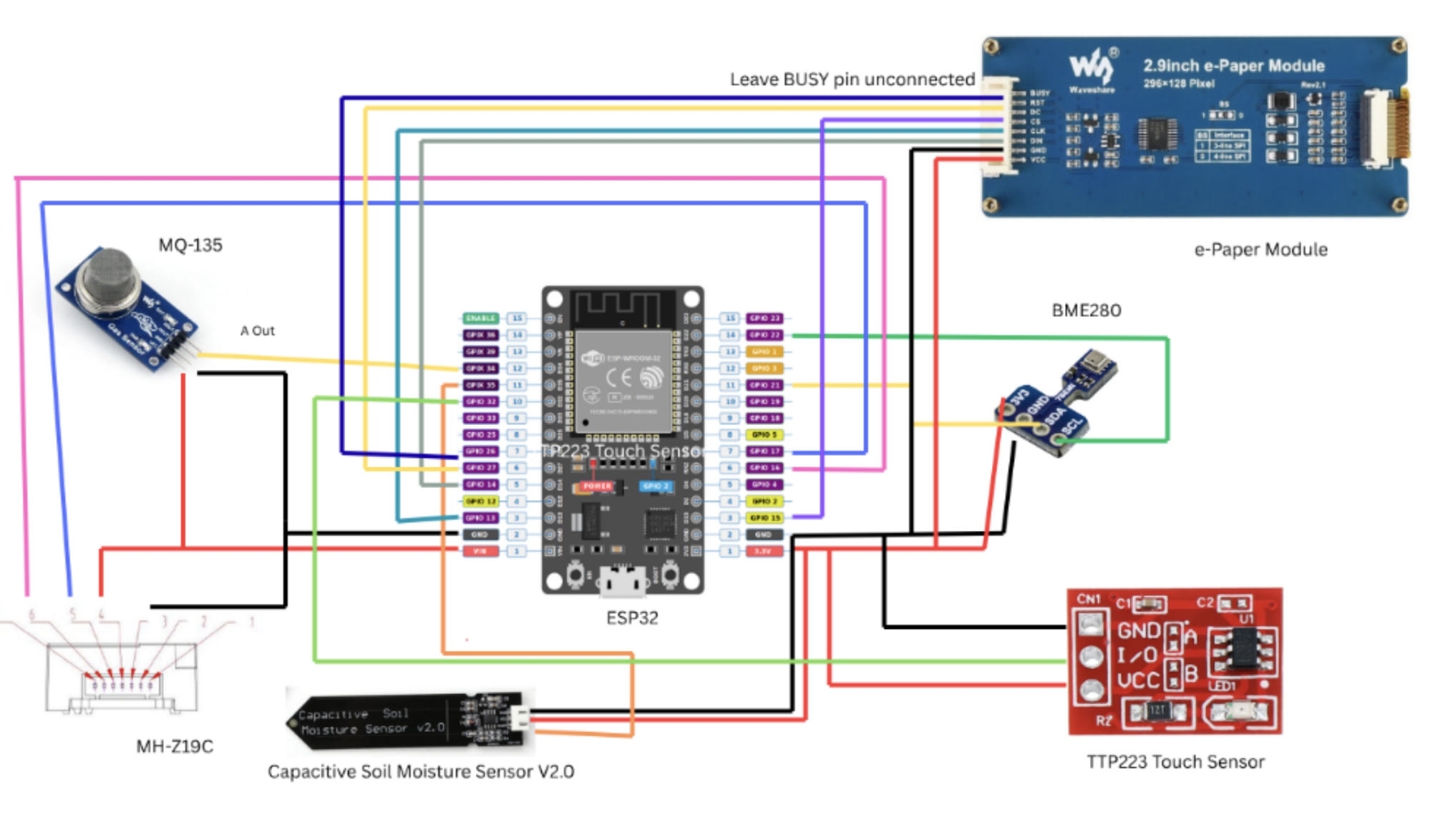
Figure 13 — Wiring diagram for the canopy (display) node: ESP32 with MQ-135, MH-Z19C, BME280, capacitive soil moisture sensor, TTP223 touch sensor, and the 2.9" e-paper display.

The power budget, in numbers

The case for a power bank over solar-plus-battery isn't a hunch - it's arithmetic. A full node (ESP32 + BME280 + MH-Z19C + MQ-135) draws about 334 mA at 5V, roughly 40 Wh a day:

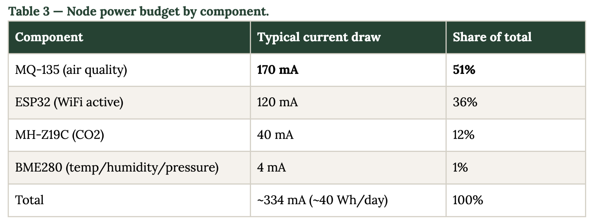
That table is the arithmetic behind "The Power Problem" above: the MQ-135's heater, not the microcontroller, decides the node's entire power story. A 10,000 mAh USB power bank, rated at its internal 3.7V cell chemistry, delivers roughly 6,500-7,000 mAh once stepped up to 5V - somewhere in the range of a full day's runtime for one node, depending on WiFi signal strength and transmit frequency. Charging it off mains power costs on the order of a few rupees a month.

Firmware: Reading BME280, MH-Z19C, and MQ-135

The following are real excerpts from the node firmware (sensor credentials replaced with placeholders for this document). Every reading cycle follows the same shape: initialise each sensor once at boot, then read all three every cycle and package them into a single InfluxDB point.

Sensor initialization (setup())

Wire.begin(BME_SDA, BME_SCL);
if (!bme.begin(0x76) && !bme.begin(0x77))
    Serial.println("ERROR: BME280 not found - check wiring");
 
co2Serial.begin(9600, SERIAL_8N1, CO2_RX_PIN, CO2_TX_PIN);
mhz19.begin(co2Serial);
mhz19.autoCalibration(false);

Reading all three sensors every cycle (loop())

float temp     = bme.readTemperature();
float humidity = bme.readHumidity();
float pressure = bme.readPressure() / 100.0f;
int   co2      = mhz19.getCO2();
int   mq135Raw = analogRead(MQ135_PIN);
 
Serial.printf("[CANOPY] %.1fC  %.0f%%RH  %.0fhPa  CO2:%dppm  AQ:%d\n",
    temp, humidity, pressure, co2, mq135Raw);

That last line is worth sitting with: the MQ-135's raw ADC value is never converted into a scientific gas concentration anywhere in the firmware or backend. It is deliberately kept as a relative number and bucketed into GOOD / FAIR / POOR bands, because the sensor itself only supports a relative claim - the same honesty the case study applies everywhere else shows up directly in this one line of code.

const char* aqLabel(int raw) {
    if (raw < 1200) return "GOOD";
    if (raw < 2500) return "FAIR";
    return "POOR";
}

The On-Node Display and the Data Pipeline

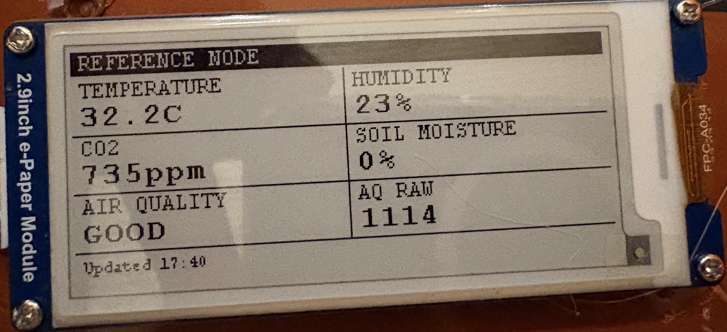
The canopy node's e-paper screen cycles through three views on a single touch of the TTP223 sensor: this node's live readings, the reference node's most recent average (fetched live over WiFi via a direct Flux query to InfluxDB), and a side-by-side bar chart comparing the two. This third screen is the plainest version of the entire project's thesis rendered in four colors on a 2.9-inch panel: a black bar for the forest, a red bar for the street, side by side, refreshed every few minutes.

struct { const char* label; float lv, rv, maxv; } g[4] = {
    { "TEMP",  localData.temp,       refData.temp,       50.0f   },
    { "HUMID", localData.hum,        refData.hum,        100.0f  },
    { "CO2",   (float)localData.co2, (float)refData.co2, 5000.0f },
    { "AQ",    (float)localData.aq,  (float)refData.aq,  4095.0f },
};

Every 5 minutes, independent of what's on screen, the node also pushes a fresh reading straight to InfluxDB over WiFi - no MQTT broker, no intermediate server, just an HTTPS write to the database. Each point carries the node's permanent UUID (generated once on first boot and stored in flash, so a node's identity survives power cycles and re-flashing), a node_type tag of canopy or reference, and the sensor fields themselves.

#define INFLUXDB_URL    "https://YOUR_INFLUXDB_HOST"
#define INFLUXDB_TOKEN  "YOUR_INFLUXDB_TOKEN"
#define INFLUXDB_ORG    "YOUR_INFLUXDB_ORG"
#define INFLUXDB_BUCKET "chhaon"
 
InfluxDBClient influx(INFLUXDB_URL, INFLUXDB_ORG, INFLUXDB_BUCKET,
                      INFLUXDB_TOKEN, InfluxDbCloud2CACert);
Point sensorPt("chhaon_readings");
 
sensorPt.clearFields();
sensorPt.addField("temperature", temp);
sensorPt.addField("humidity",    humidity);
sensorPt.addField("pressure",    pressure);
sensorPt.addField("co2",         co2);
sensorPt.addField("mq135_raw",   mq135Raw);
sensorPt.addField("rssi_dbm",    (int)WiFi.RSSI());
influx.writePoint(sensorPt);

InfluxDB itself isn't an arbitrary choice either. It's a time-series database, purpose-built for exactly this shape of data: a timestamp, a small set of numeric fields, and tags to slice by - which is precisely what "a CO2 reading every 5 minutes, forever, from two node types" looks like. A general-purpose database would work, but would need to be taught to do efficiently what a time-series database does by default: range queries over time windows, downsampling, and retention policies. That last point matters more than it sounds. A forest's carbon story is only provable with a long, unbroken history - a single day's reading proves nothing, but 6-12 months of continuous, paired-node data is what a carbon registry actually wants to see. That single requirement is the real reason this whole pipeline exists in its current shape, and it's the bridge into the next section: how that stream of temperature and CO2 numbers becomes a carbon credit calculation.

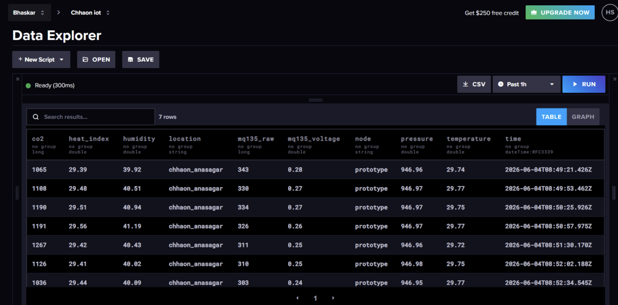
Figure 8 — Live sensor data in InfluxDB Cloud's Data Explorer (the "chhaon_anasagar" prototype node).

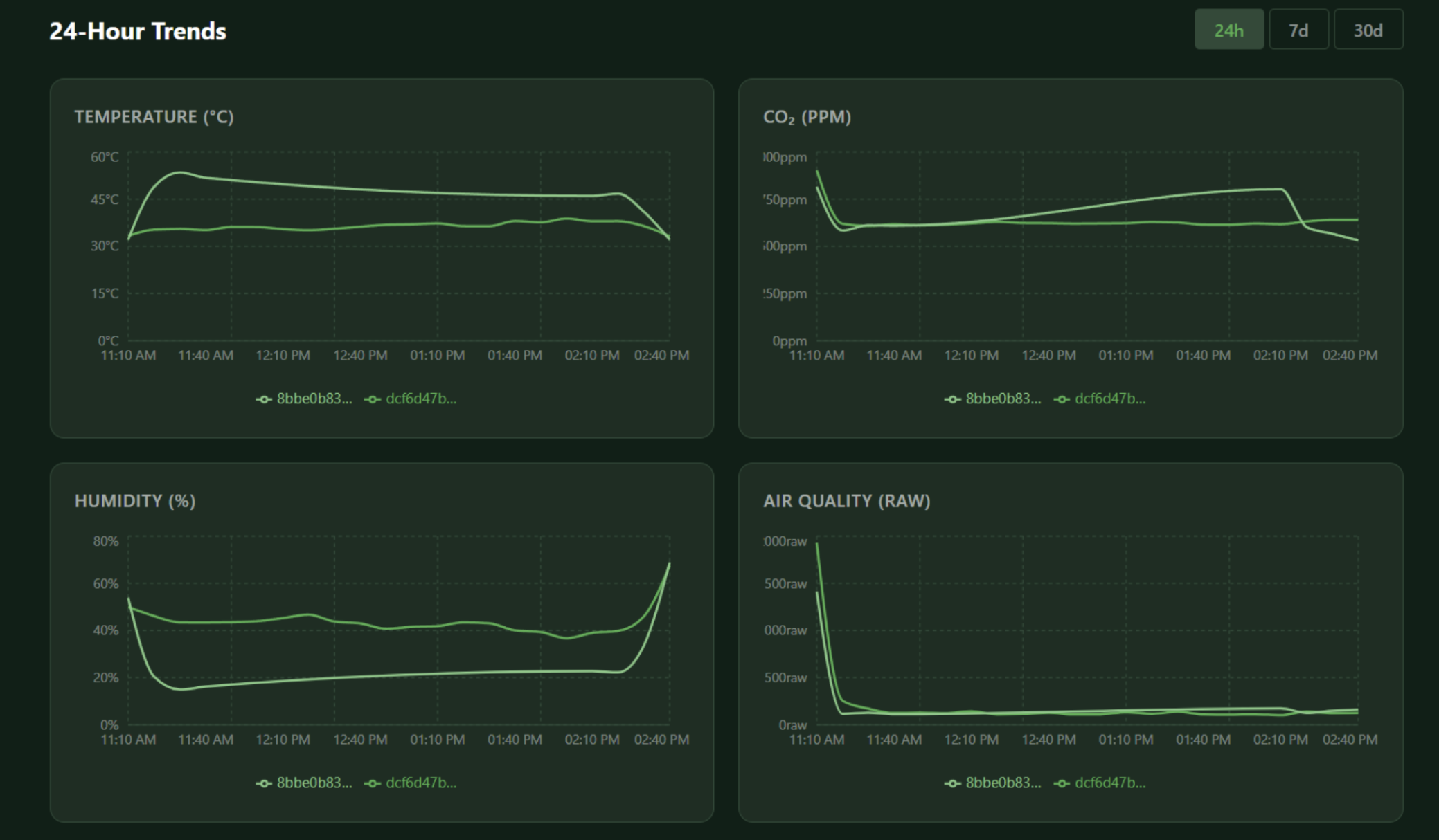
Figure 9 — The web dashboard's 24-hour trend view, comparing two nodes across temperature, CO2, humidity, and air quality.

The Carbon Credit Algorithm

"Turning Readings Into Meaning" (above) describes the carbon accounting logic in plain language. This section is its technical reference: the full set of symbols, formulas, and worked numbers a backend engineer would need to implement or audit the pipeline. It follows the project's internal algorithm reference document (CHLSPOT-ALG-001) step for step. As with the rest of this case study, worked examples below use representative numbers to demonstrate how the math works, not confirmed measurements from the Ajmer site - that distinction is called out again at the end of this section.

Definitions and Symbols

All formulas in this section use the symbols below, in SI units. Any conversion from a device's native reporting unit happens once, at ingest.

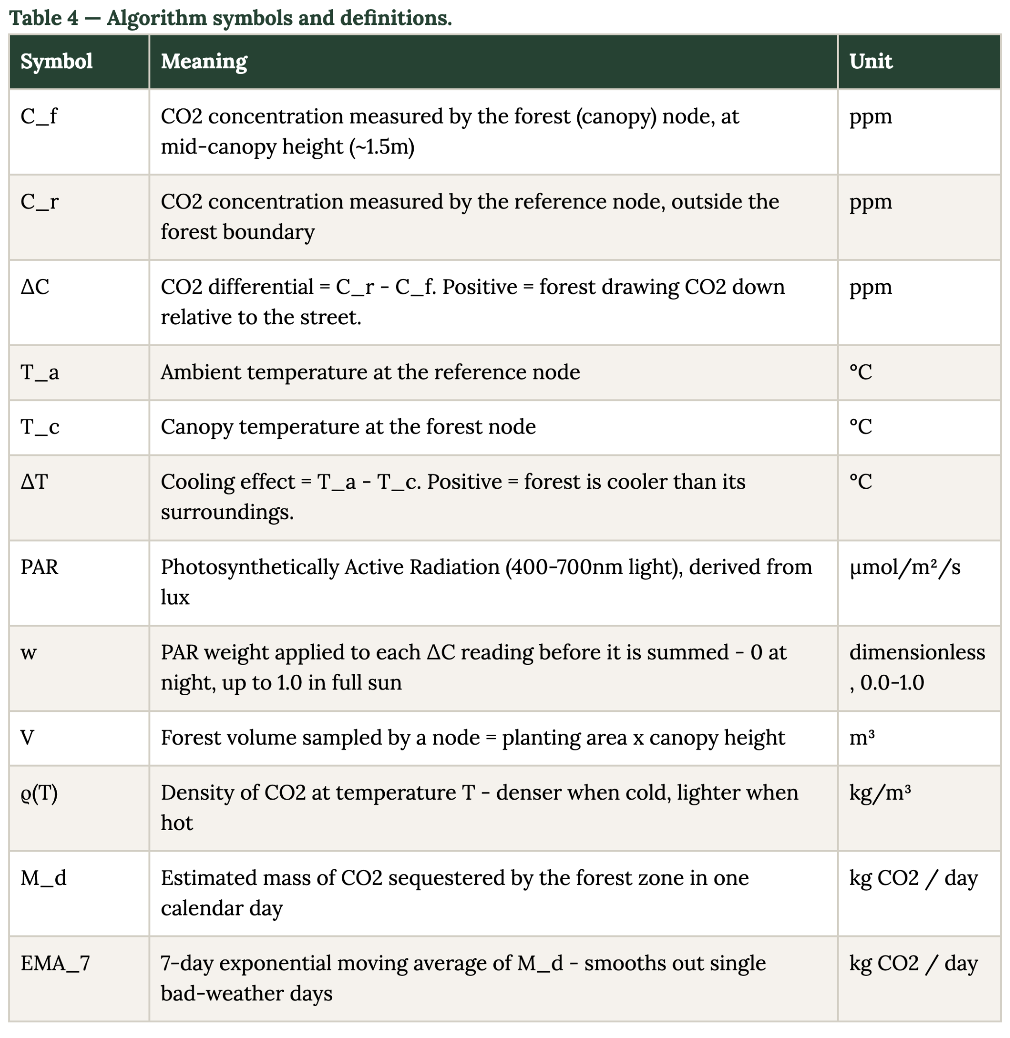
Node Roles: Forest vs. Reference

The entire algorithm rests on one distinction: every reading is either from a forest (canopy) node or a reference node, and the computation always compares one against the other - never either one alone.

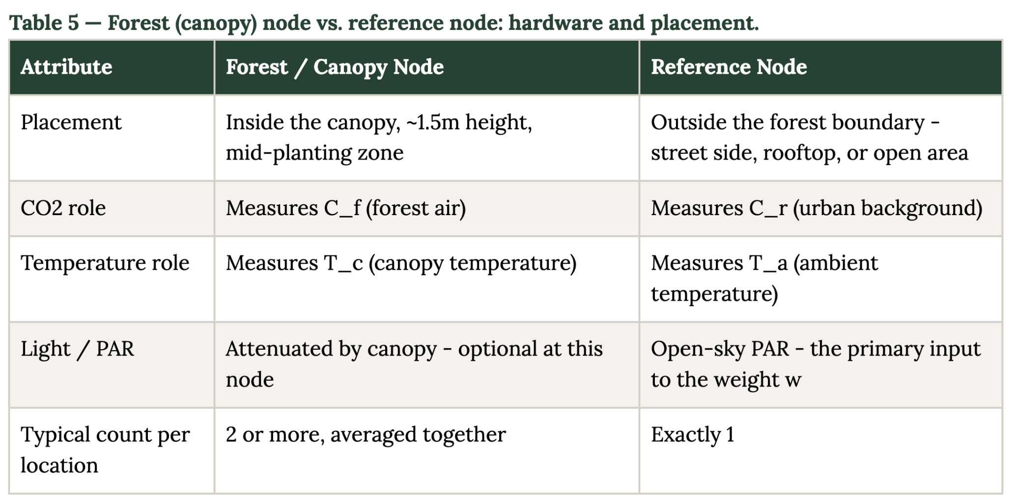
Why averaging matters

When a location has more than one forest node, their ΔC values are averaged before the mass conversion in Step 4 - and any node flagged as an anomaly or offline is excluded from that average rather than dragging the whole reading down.

Step-by-Step Computation

Step 1 - Ingestion and Validation

Every inbound reading passes three checks before it enters the pipeline as status "ok": the device ID and timestamp must be well-formed; each sensor value must fall inside a physically plausible range (CO2 300-5000ppm, temperature -10 to 60°C, humidity 0-100%, PAR 0-2500µmol/m²/s); and the device's clock must not have drifted more than 300 seconds from the server's. A reading that fails a check is still stored, tagged with its failure reason, but excluded from computation until cleared - a single bad CO2 spike doesn't throw away that packet's perfectly good temperature and humidity values.

Step 2 - Differential Computation (ΔC and ΔT)

For every valid forest-node reading, the backend pairs it with the most recent reference-node reading from the same location, within a 10-minute window.

Formula

ΔC = C_r - C_f          // positive = sequestration signal
ΔT = T_a - T_c          // positive = cooling / UHI offset
ΔC_avg = (ΔC_node1 + ΔC_node2 + ... + ΔC_nodeN) / N   // multi-node average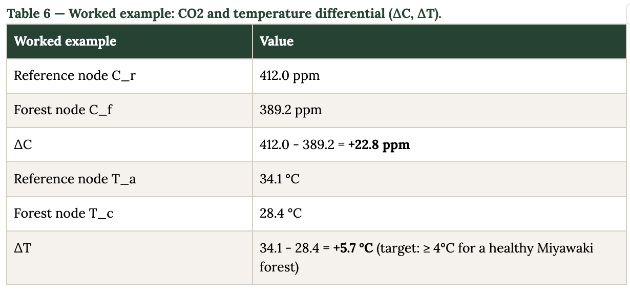

Step 3 - PAR Weighting

Plants only sequester CO2 through photosynthesis, which requires light - so a nighttime reading, where CO2 is naturally elevated under the canopy from plant respiration, must not be allowed to count as "no capture" or worse, count negatively against the day's total. Each ΔC reading is weighted by how much usable light was available at that moment, measured at the reference node's open sky (canopy light is attenuated by the forest itself and would undercount what's driving photosynthesis higher up).

Formula

w = min(1.0, PAR_ref / 400)     // 400 µmol/m²/s = light saturation point, most C3 plants
ΔC_w[i] = ΔC_avg[i] x w[i]
 
// w = 0.0 at night or heavy overcast -> reading contributes zero
// w = 0.5 at ~200 µmol/m²/s (heavy cloud)
// w = 1.0 at ≥ 400 µmol/m²/s (clear sun)

Step 4 - CO2 Mass Conversion

This is the step that turns a ppm differential into an actual weight of gas, and it's also where local climate enters the math directly: CO2 is measurably denser on a cool morning than on a 45°C summer afternoon, so density is computed per reading rather than assumed constant.

Formula

// 1. CO2 density at canopy temperature (ideal gas law)
ρ(T_c) = (44.01 / 22.4) x (273.15 / (273.15 + T_c))     // kg/m³
 
// 2. Forest air volume (from the devices table, updated every 6 months)
V = planting_area_m2 x canopy_height_m
 
// 3. Daily sequestration mass - summed across every reading in the day
contribution_i = (ΔC_w[i] / 1,000,000) x V x ρ(T_c[i]) x h_i
M_d = Σ contribution_i     // kg CO2 / day
// h_i = reading interval in hours (e.g. 5-min cycle -> h_i = 300/3600 = 0.0833 hr)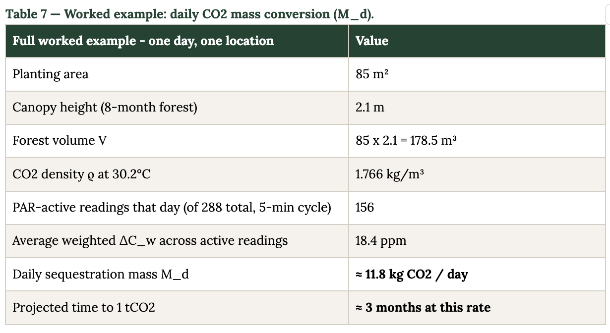

Why the density correction matters here

CO2 density works out to about 1.868 kg/m³ at 15°C and 1.690 kg/m³ at 45°C - a 10.5% swing across a Rajasthan year. Skipping this correction and using one fixed density would systematically overstate summer sequestration relative to winter. The algorithm also notes an elevation/pressure correction (multiplying ρ by the local-to-sea-level pressure ratio) for registry-grade accuracy, since both Jaipur and Ajmer sit several hundred metres above sea level.

Step 5 - Rolling Aggregation and Smoothing

A single day's M_d is too noisy to report on its own - a dust storm or a cloudy monsoon day can make a healthy forest look like it stopped sequestering for a day. Two smoothing mechanisms handle this.

Formula

monthly_tCO2 = Σ M_d[last 30 days] / 1000       // reported figure
 
// 7-day exponential moving average, alpha = 2/(7+1) = 0.25
EMA_7[today] = 0.25 x M_d[today] + 0.75 x EMA_7[yesterday]
 
// Guardrail: no single day may move the 30-day rolling total by more than +-15%
// A day that would breach this is capped; the capped value (not the raw one) is used

Step 6 - Credit Issuance Trigger

Carbon registries such as Verra VCS and Gold Standard issue credits in whole tonnes, so the backend simply accumulates daily M_d values per location until the running total crosses 1.0 tCO2 - and only then, if data completeness for that period is also at least 85%, does it flag a batch for a human admin to review and manually submit. That last step is deliberately not automated: a person checks the batch before it ever reaches a registry.

Formula

IF running_tCO2 >= 1.0 AND data_completeness_pct >= 85:
    -> create a pending carbon_credit_batch, notify admin
ELSE IF data_completeness_pct < 85:
    -> flag "insufficient_data" - batch withheld regardless of tCO2 total

The 85% completeness floor exists because partial data quietly inflates apparent sequestration - a location with chronic sensor outages tends to be missing exactly its lowest-performing hours, not a random sample. A new location also runs for its first 60 days in an observational-only mode: every value is computed and stored normally, but nothing from that window counts toward a credit batch, giving the team real data to validate the model's constants before trusting them.

Handling Anomalies, Data Gaps, and Calibration

Sensors drift, get dusty, and occasionally fail - the pipeline is built to expect that rather than be surprised by it.

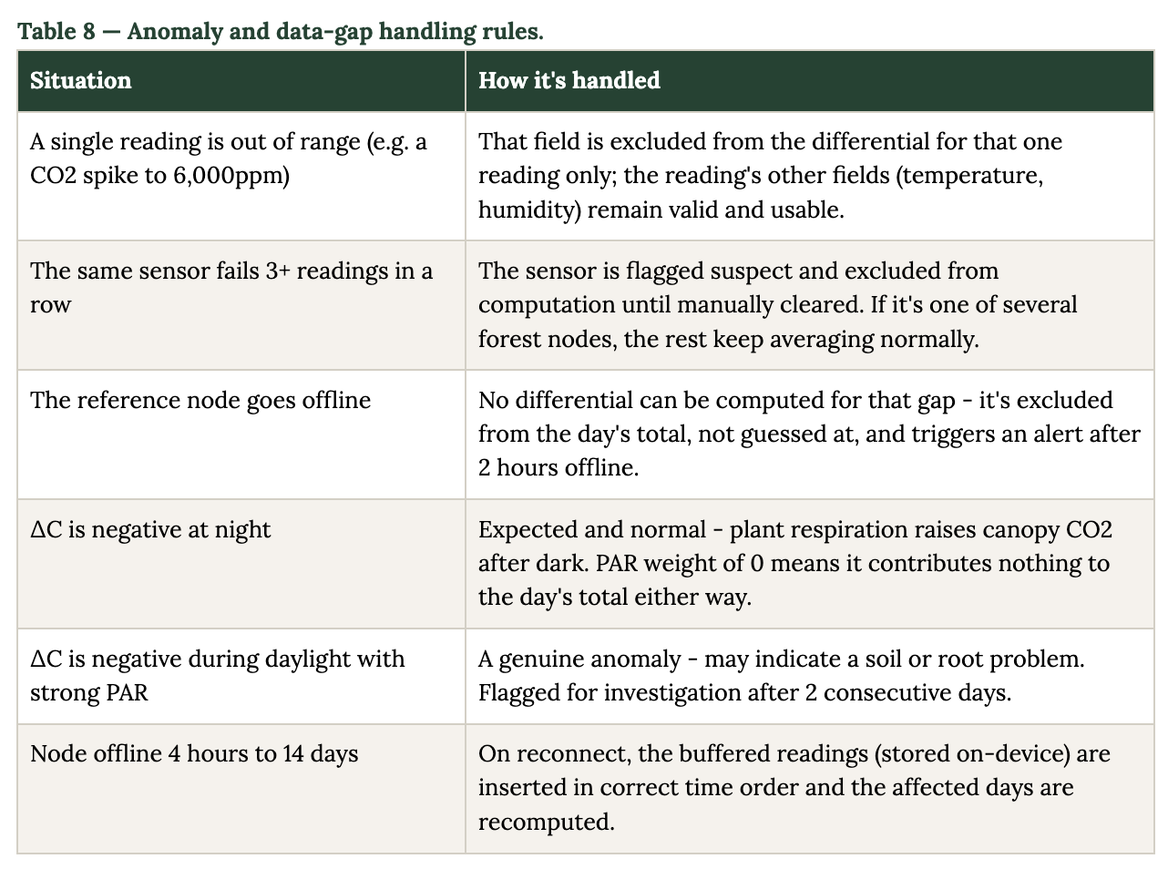
The formula constants used throughout this section - the 400 µmol/m²/s PAR saturation point, the 4°C cooling target, the 25 ppm CO2 capture target, the 85% completeness floor - are documented starting points from plant-physiology literature and Miyawaki forest studies, not numbers unique to Ajmer. The algorithm reference explicitly calls for calibrating them against 60+ days of real site data before the first credit batch is ever submitted.

Proving It: Forest vs. Street, Cooler and Cleaner

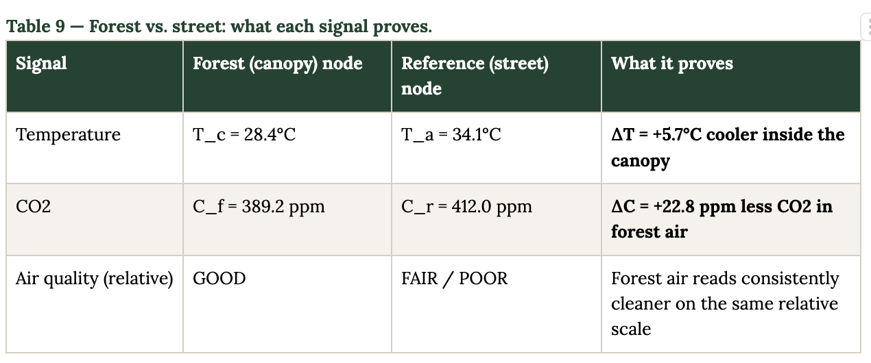
All of the engineering above exists to answer one visitor-facing question: is it actually different in here? Not "does it feel cooler" - a number, computed the same way every time, from two sensors that never move. This section pulls together the same ΔT and ΔC signals used for the carbon calculation and shows how they're already being used to demonstrate, live, that the forest runs cooler and cleaner than the street beside it - and where that comparison shows up today versus where it's headed.

The Cooling Proof

ΔT (ambient minus canopy temperature) is reused here as the headline cooling claim. In the worked example earlier in this document, a reference (street-side) node reading 34.1°C alongside a canopy reading of 28.4°C produces a ΔT of +5.7°C - a forest running nearly 6 degrees cooler than the pavement a few metres away, at the same moment, measured by hardware that never moves between the two spots. That "same moment, same method, every time" property is exactly what a skeptic-proof measurement needs and what a single walk-around thermometer reading can never offer.

The Air Quality Proof

Air quality works the same way but leans on two different signals rather than one: the CO2 differential (ΔC) already used for carbon accounting, and the MQ-135's relative GOOD / FAIR / POOR band, compared side by side between the two nodes. Because the MQ-135 doesn't report a scientific concentration, the comparison deliberately stays qualitative - the claim being made is "the street reads worse than the forest, consistently," not a specific pollutant figure. That's a smaller claim than a lab-grade air-quality index would allow, and it's also one this hardware can actually back up.

Where the Comparison Gets Displayed

This comparison already exists in two places, at two different levels of polish:

1. On the node itself, today: the e-paper display's third screen (shown earlier in this section) renders exactly this comparison as a black-bar-versus-red-bar chart for temperature, humidity, CO2, and air quality, refreshed every few minutes, visible to anyone standing in front of the node without needing a phone or an app.

2. On a public dashboard:

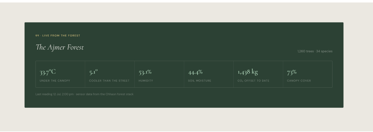
Figure 10 — Concept mockup of the public dashboard card, showing the forest-vs-street comparison stats.

The point of building it this way

A single sensor reading is an assertion. A paired reading, taken the same way at the same moment by hardware that never changes position, is evidence. Everything in this section and the two before it exists to move Chhaon's central claim - that this forest is measurably cooler and cleaner than the street beside it - from something visitors are told to something they can check for themselves.

Challenges

Sourcing Parts That Don't Exist Locally

None of the specific sensors Chhaon needed were sitting on a shelf in Ajmer. The team had to order every one of them from two Indian electronics component websites, Robocraze and Robu, and wait for shipping before any real prototyping could start.

The E-Paper Display Not Working

The node's small e-paper display, a four-color Waveshare panel, refused to show a single reading at first. The standard library everyone expected to just work didn't fetch data correctly. The team spent two to three days digging through GitHub repositories and other people's code examples before finding a driver that actually worked with this specific panel.

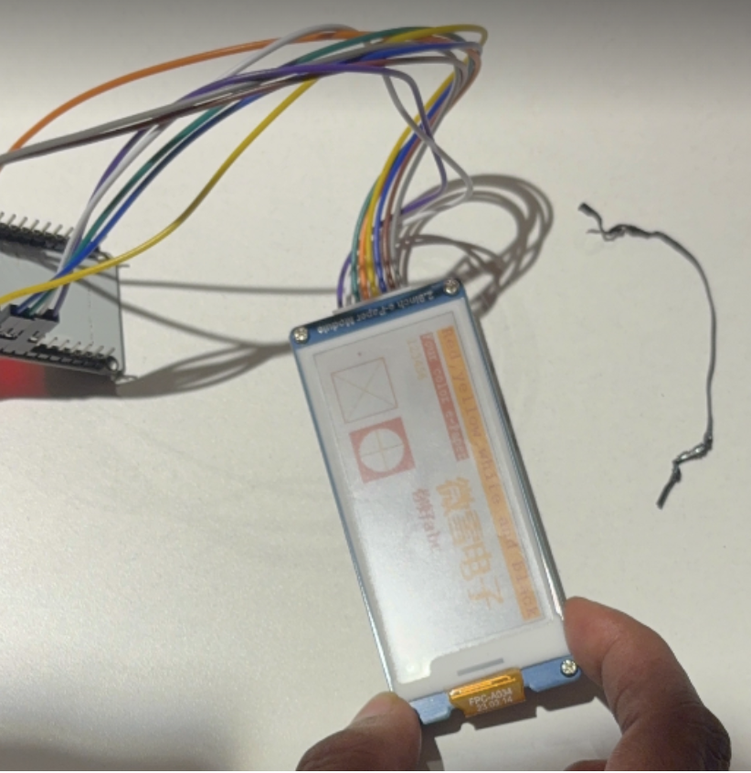
Figure 14— The Waveshare 2.9" e-paper display during driver debugging.

The Plastic Box

The first home the team built for a sensor node was a plastic storage box. They cut holes into it by hand and soldered wiring through those holes to get sensors and cables in and out. Indoors, it worked fine. Outdoors, it never stood a chance. The same holes that let wires through also let rain in, and Ajmer's dust storms found their way inside a box that was never sealed for weather in the first place.

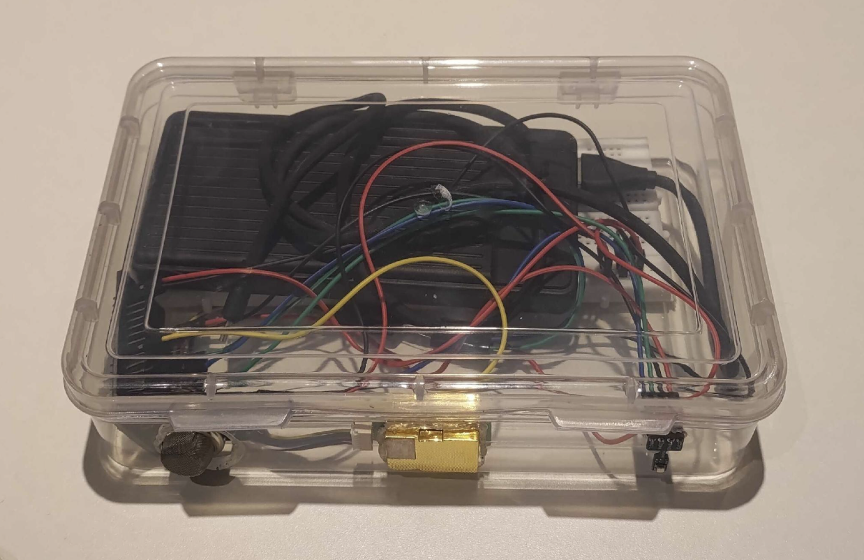
Figure 15 — The original plastic-box enclosure prototype, wired and tested indoors.

Building It Properly, With a Carpenter

To actually fix the weatherproofing problem, the team went to a local carpenter, and asked for a demo wooden enclosure made from MDF board, briefed specifically to survive real outdoor conditions, not just look finished in a photo.

The Day It Rained

On the day the team set up both nodes together, the reference node and the canopy node, side by side, it rained hard in Ajmer. To get the reference node some height off the ground, the team propped it up on a wooden slate. The storm soaked that slate straight through. Moisture crept up into the CO2 sensor sitting on top of it, and the sensor started malfunctioning within hours.

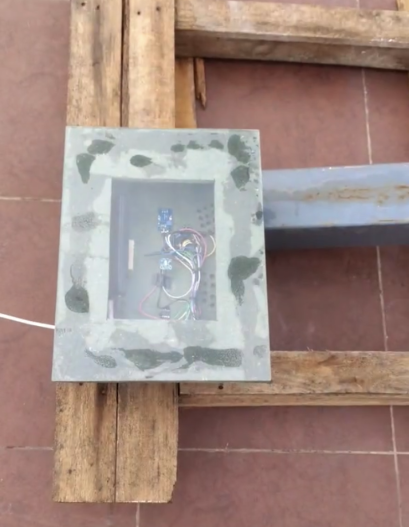
Figure 16 — The reference node's outdoor enclosure, mounted on the wooden slate that let rain reach the CO2 sensor.

What We're Building Now

The current enclosure design draws on the Davis Radiation Shield, a well-known weather-instrument shield design. The exact material that design calls for wasn't easy to source locally, so the team improvised: pot plates, linked together with plastic back-scratchers acting as connecting rods, five or six plates stacked to form a shield around the sensors.

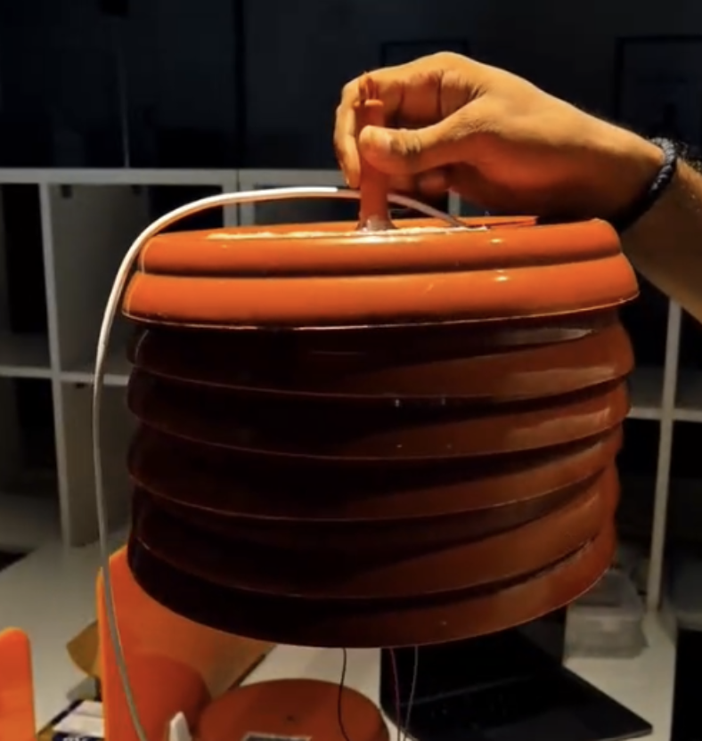
Figure 17 — The current enclosure prototype: stacked pot plates forming a Davis Radiation Shield-style cover.

Every one of these moments — the plastic box, the hunt for parts on Robocraze and Robu, the wooden enclosure, the ruined CO2 sensor, the shield made from pot plates — taught the same lesson from a different angle: a sensor sitting outdoors in Ajmer has to survive Ajmer, not a lab.

Why This Approach Works

• Prove it, don't just plant it. Anyone can put a sapling in the ground and call it climate action. Chhaon pairs every plant with a live measurement of what that plant is actually doing, which turns a claim into something a stranger can check for themselves.

• Build small first, then build real. The drum, the terrace node, the demo wooden box, the single working sensor node: none of these were the finished product, and none of them were meant to be. Each one answered one question cheaply before the team spent real money finding out the hard way.

• Native species and honest data are the same instinct. Refusing to plant anything that isn't native to Rajasthan, and refusing to report a sensor reading the hardware can't actually back up, come from the same place: a preference for what's real over what looks good.

Key Lessons From This Project

• Weatherproofing has to be tested, not assumed. A box that survives a living room doesn't survive a monsoon. Only real rain and real dust proved that, not a spec sheet.

• Local sourcing constraints shape what your hardware plan can actually be. When a part doesn't exist in local shops, or a nursery doesn't carry the species you need, the plan bends around that reality, and the finished project is better for having bent early.

• The power-hungry part of a system isn't always the one you'd guess. Nobody assumes an air quality sensor's internal heater would outdraw a processor. It does, and designing around that fact matters more than designing around the part that looks technical.

• A scaled-down first version is not a failure, it's a decision. Shipping four honest sensors instead of eight ambitious ones wasn't a compromise. It was the difference between a real instrument in the ground and a wish list still sitting on a slide.

• A measurement only matters if it can't be faked by accident. Paired nodes, sunlight weighting, anomaly caps, and a completeness threshold all exist for one reason: so a good number means the forest is actually working, not that the weather happened to cooperate for a day.

Conclusion

Ajmer has always known that shade helps. What it never had was a way to prove it — one sensor reading at a time. Chhaon is that proof, still being built. The forest is growing in its containers on the fifth floor. The sensors are running, paired, and recording. The math behind the carbon accounting works on paper and in code. What's still ahead is the part everyone will eventually see: a public dashboard showing live numbers instead of placeholders, and real submissions to the carbon registries this system was designed for.

The difference between a city that endures its summers and one that starts measuring its way out of them isn't a bigger idea. It's smaller than that. It's a sensor under a tree, a number on a screen, and someone willing to check it.

A note on where things stand: the sensor hardware, the firmware, and the carbon-accounting logic described in this piece are real, built, and running today. The public-facing dashboard is currently displaying well-built placeholder data while the live pipeline from the sensors is being connected, and no real carbon credit batch has been submitted to any registry yet. Both are the project's next milestones, not results already achieved.